Run this notebook online:![]() or Colab:
or Colab: ![]()
7.3. Network in Network (NiN)
LeNet, AlexNet, and VGG all share a common design pattern: extract features exploiting spatial structure via a sequence of convolutions and pooling layers and then post-process the representations via fully-connected layers. The improvements upon LeNet by AlexNet and VGG mainly lie in how these later networks widen and deepen these two modules. Alternatively, one could imagine using fully-connected layers earlier in the process. However, a careless use of dense layers might give up the spatial structure of the representation entirely, Network in Network (NiN) blocks offer an alternative. They were proposed in [Lin et al., 2013] based on a very simple insight—to use an MLP on the channels for each pixel separately.
7.3.1. NiN Blocks
Recall that the inputs and outputs of convolutional layers consist of four-dimensional arrays with axes corresponding to the batch, channel, height, and width. Also recall that the inputs and outputs of fully-connected layers are typically two-dimensional arrays corresponding to the batch, and features. The idea behind NiN is to apply a fully-connected layer at each pixel location (for each height and width). If we tie the weights across each spatial location, we could think of this as a \(1\times 1\) convolutional layer (as described in Section 6.4) or as a fully-connected layer acting independently on each pixel location. Another way to view this is to think of each element in the spatial dimension (height and width) as equivalent to an example and the channel as equivalent to a feature. Fig. 7.3.1 illustrates the main structural differences between NiN and AlexNet, VGG, and other networks.

Fig. 7.3.1 The figure on the left shows the network structure of AlexNet and VGG, and the figure on the right shows the network structure of NiN.
The NiN block consists of one convolutional layer followed by two \(1\times 1\) convolutional layers that act as per-pixel fully-connected layers with ReLU activations. The convolution width of the first layer is typically set by the user. The subsequent widths are fixed to \(1 \times 1\).
%load ../utils/djl-imports
%load ../utils/plot-utils
%load ../utils/Training.java
%load ../utils/Accumulator.java
import ai.djl.basicdataset.cv.classification.*;
import ai.djl.metric.*;
import org.apache.commons.lang3.ArrayUtils;
// setting the seed for demonstration purpose. You can remove it when you run the notebook
Engine.getInstance().setRandomSeed(5555);

public SequentialBlock niNBlock(int numChannels, Shape kernelShape,
                     Shape strideShape, Shape paddingShape){

    SequentialBlock tempBlock = new SequentialBlock();

    tempBlock.add(Conv2d.builder()
              .setKernelShape(kernelShape)
              .optStride(strideShape)
              .optPadding(paddingShape)
              .setFilters(numChannels)
              .build())
        .add(Activation::relu)
        .add(Conv2d.builder()
              .setKernelShape(new Shape(1, 1))
              .setFilters(numChannels)
              .build())
        .add(Activation::relu)
        .add(Conv2d.builder()
              .setKernelShape(new Shape(1, 1))
              .setFilters(numChannels)
              .build())
        .add(Activation::relu);

    return tempBlock;
}
7.3.2. NiN Model
The original NiN network was proposed shortly after AlexNet and clearly draws some inspiration. NiN uses convolutional layers with window shapes of \(11\times 11\), \(5\times 5\), and \(3\times 3\), and the corresponding numbers of output channels are the same as in AlexNet. Each NiN block is followed by a maximum pooling layer with a stride of 2 and a window shape of \(3\times 3\).
Once significant difference between NiN and AlexNet is that NiN avoids dense connections altogether. Instead, NiN uses an NiN block with a number of output channels equal to the number of label classes, followed by a global average pooling layer, yielding a vector of logits. One advantage of NiN’s design is that it significantly reduces the number of required model parameters. However, in practice, this design sometimes requires increased model training time.
SequentialBlock block = new SequentialBlock();

block.add(niNBlock(96, new Shape(11, 11), new Shape(4, 4), new Shape(0, 0)))
     .add(Pool.maxPool2dBlock(new Shape(3, 3), new Shape(2, 2)))
     .add(niNBlock(256, new Shape(5, 5), new Shape(1, 1), new Shape(2, 2)))
     .add(Pool.maxPool2dBlock(new Shape(3, 3), new Shape(2, 2)))
     .add(niNBlock(384, new Shape(3, 3), new Shape(1, 1), new Shape(1, 1)))
     .add(Pool.maxPool2dBlock(new Shape(3, 3), new Shape(2, 2)))
     .add(Dropout.builder().optRate(0.5f).build())
     // There are 10 label classes
     .add(niNBlock(10, new Shape(3, 3), new Shape(1, 1), new Shape(1, 1)))
     // The global average pooling layer automatically sets the window shape
     // to the height and width of the input
     .add(Pool.globalAvgPool2dBlock())
     // Transform the four-dimensional output into two-dimensional output
     // with a shape of (batch size, 10)
     .add(Blocks.batchFlattenBlock());
SequentialBlock {
    SequentialBlock {
            Conv2d
            LambdaBlock
            Conv2d
            LambdaBlock
            Conv2d
            LambdaBlock
    }
    maxPool2d
    SequentialBlock {
            Conv2d
            LambdaBlock
            Conv2d
            LambdaBlock
            Conv2d
            LambdaBlock
    }
    maxPool2d
    SequentialBlock {
            Conv2d
            LambdaBlock
            Conv2d
            LambdaBlock
            Conv2d
            LambdaBlock
    }
    maxPool2d
    Dropout
    SequentialBlock {
            Conv2d
            LambdaBlock
            Conv2d
            LambdaBlock
            Conv2d
            LambdaBlock
    }
    globalAvgPool2d
    batchFlatten
}
We create a data example to see the output shape of each block.
float lr = 0.1f;
Model model = Model.newInstance("cnn");
model.setBlock(block);

Loss loss = Loss.softmaxCrossEntropyLoss();

Tracker lrt = Tracker.fixed(lr);
Optimizer sgd = Optimizer.sgd().setLearningRateTracker(lrt).build();

DefaultTrainingConfig config = new DefaultTrainingConfig(loss).optOptimizer(sgd) // Optimizer (loss function)
                .optDevices(Engine.getInstance().getDevices(1)) // single GPU
                .addEvaluator(new Accuracy()) // Model Accuracy
                .addTrainingListeners(TrainingListener.Defaults.logging()); // Logging

Trainer trainer = model.newTrainer(config);

NDManager manager = NDManager.newBaseManager();
NDArray X = manager.randomUniform(0f, 1.0f, new Shape(1, 1, 224, 224));
trainer.initialize(X.getShape());

Shape currentShape = X.getShape();

for (int i = 0; i < block.getChildren().size(); i++) {

    Shape[] newShape = block.getChildren().get(i).getValue().getOutputShapes(new Shape[]{currentShape});
    currentShape = newShape[0];
    System.out.println(block.getChildren().get(i).getKey() + " layer output : " + currentShape);
}
INFO Training on: 1 GPUs.
INFO Load MXNet Engine Version 1.9.0 in 0.074 ms.
01SequentialBlock layer output : (1, 96, 54, 54)
02LambdaBlock layer output : (1, 96, 26, 26)
03SequentialBlock layer output : (1, 256, 26, 26)
04LambdaBlock layer output : (1, 256, 12, 12)
05SequentialBlock layer output : (1, 384, 12, 12)
06LambdaBlock layer output : (1, 384, 5, 5)
07Dropout layer output : (1, 384, 5, 5)
08SequentialBlock layer output : (1, 10, 5, 5)
09LambdaBlock layer output : (1, 10)
10LambdaBlock layer output : (1, 10)
7.3.3. Data Acquisition and Training
As before we use Fashion-MNIST to train the model. NiN’s training is similar to that for AlexNet and VGG, but it often uses a larger learning rate.
int batchSize = 128;
int numEpochs = Integer.getInteger("MAX_EPOCH", 10);

double[] trainLoss;
double[] testAccuracy;
double[] epochCount;
double[] trainAccuracy;

epochCount = new double[numEpochs];

for (int i = 0; i < epochCount.length; i++) {
    epochCount[i] = i+1;
}

FashionMnist trainIter = FashionMnist.builder()
        .addTransform(new Resize(224))
        .addTransform(new ToTensor())
        .optUsage(Dataset.Usage.TRAIN)
        .setSampling(batchSize, true)
        .optLimit(Long.getLong("DATASET_LIMIT", Long.MAX_VALUE))
        .build();

FashionMnist testIter = FashionMnist.builder()
        .addTransform(new Resize(224))
        .addTransform(new ToTensor())
        .optUsage(Dataset.Usage.TEST)
        .setSampling(batchSize, true)
        .optLimit(Long.getLong("DATASET_LIMIT", Long.MAX_VALUE))
        .build();

trainIter.prepare();
testIter.prepare();
Map<String, double[]> evaluatorMetrics = new HashMap<>();
double avgTrainTimePerEpoch = Training.trainingChapter6(trainIter, testIter, numEpochs, trainer, evaluatorMetrics);
Training:    100% |████████████████████████████████████████| Accuracy: 0.36, SoftmaxCrossEntropyLoss: 1.65
Validating:  100% |████████████████████████████████████████|
INFO Epoch 1 finished.
INFO Train: Accuracy: 0.36, SoftmaxCrossEntropyLoss: 1.65
INFO Validate: Accuracy: 0.21, SoftmaxCrossEntropyLoss: 2.29
Training:    100% |████████████████████████████████████████| Accuracy: 0.64, SoftmaxCrossEntropyLoss: 0.93
Validating:  100% |████████████████████████████████████████|
INFO Epoch 2 finished.
INFO Train: Accuracy: 0.64, SoftmaxCrossEntropyLoss: 0.93
INFO Validate: Accuracy: 0.72, SoftmaxCrossEntropyLoss: 0.71
Training:    100% |████████████████████████████████████████| Accuracy: 0.74, SoftmaxCrossEntropyLoss: 0.66
Validating:  100% |████████████████████████████████████████|
INFO Epoch 3 finished.
INFO Train: Accuracy: 0.74, SoftmaxCrossEntropyLoss: 0.66
INFO Validate: Accuracy: 0.79, SoftmaxCrossEntropyLoss: 0.58
Training:    100% |████████████████████████████████████████| Accuracy: 0.77, SoftmaxCrossEntropyLoss: 0.63
Validating:  100% |████████████████████████████████████████|
INFO Epoch 4 finished.
INFO Train: Accuracy: 0.77, SoftmaxCrossEntropyLoss: 0.63
INFO Validate: Accuracy: 0.77, SoftmaxCrossEntropyLoss: 0.66
Training:    100% |████████████████████████████████████████| Accuracy: 0.82, SoftmaxCrossEntropyLoss: 0.49
Validating:  100% |████████████████████████████████████████|
INFO Epoch 5 finished.
INFO Train: Accuracy: 0.82, SoftmaxCrossEntropyLoss: 0.49
INFO Validate: Accuracy: 0.84, SoftmaxCrossEntropyLoss: 0.46
Training:    100% |████████████████████████████████████████| Accuracy: 0.79, SoftmaxCrossEntropyLoss: 0.61
Validating:  100% |████████████████████████████████████████|
INFO Epoch 6 finished.
INFO Train: Accuracy: 0.79, SoftmaxCrossEntropyLoss: 0.61
INFO Validate: Accuracy: 0.82, SoftmaxCrossEntropyLoss: 0.50
Training:    100% |████████████████████████████████████████| Accuracy: 0.84, SoftmaxCrossEntropyLoss: 0.44
Validating:  100% |████████████████████████████████████████|
INFO Epoch 7 finished.
INFO Train: Accuracy: 0.84, SoftmaxCrossEntropyLoss: 0.44
INFO Validate: Accuracy: 0.85, SoftmaxCrossEntropyLoss: 0.44
Training:    100% |████████████████████████████████████████| Accuracy: 0.86, SoftmaxCrossEntropyLoss: 0.39
Validating:  100% |████████████████████████████████████████|
INFO Epoch 8 finished.
INFO Train: Accuracy: 0.86, SoftmaxCrossEntropyLoss: 0.39
INFO Validate: Accuracy: 0.87, SoftmaxCrossEntropyLoss: 0.36
Training:    100% |████████████████████████████████████████| Accuracy: 0.87, SoftmaxCrossEntropyLoss: 0.35
Validating:  100% |████████████████████████████████████████|
INFO Epoch 9 finished.
INFO Train: Accuracy: 0.87, SoftmaxCrossEntropyLoss: 0.35
INFO Validate: Accuracy: 0.87, SoftmaxCrossEntropyLoss: 0.36
Training:    100% |████████████████████████████████████████| Accuracy: 0.88, SoftmaxCrossEntropyLoss: 0.33
Validating:  100% |████████████████████████████████████████|
INFO Epoch 10 finished.
INFO Train: Accuracy: 0.88, SoftmaxCrossEntropyLoss: 0.33
INFO Validate: Accuracy: 0.88, SoftmaxCrossEntropyLoss: 0.34
trainLoss = evaluatorMetrics.get("train_epoch_SoftmaxCrossEntropyLoss");
trainAccuracy = evaluatorMetrics.get("train_epoch_Accuracy");
testAccuracy = evaluatorMetrics.get("validate_epoch_Accuracy");

System.out.printf("loss %.3f,", trainLoss[numEpochs - 1]);
System.out.printf(" train acc %.3f,", trainAccuracy[numEpochs - 1]);
System.out.printf(" test acc %.3f\n", testAccuracy[numEpochs - 1]);
System.out.printf("%.1f examples/sec", trainIter.size() / (avgTrainTimePerEpoch / Math.pow(10, 9)));
System.out.println();
loss 0.332, train acc 0.879, test acc 0.879
2598.5 examples/sec
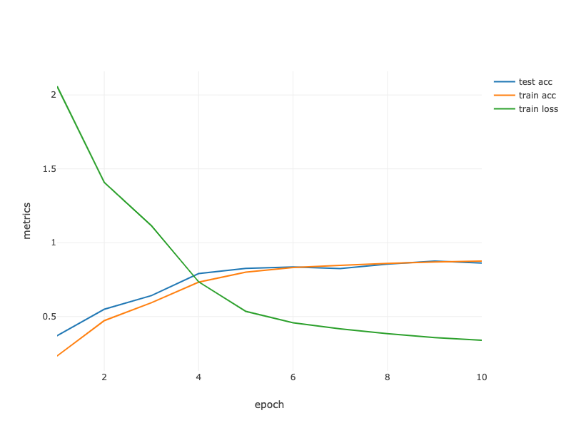
Fig. 7.3.2 Contour Gradient Descent.
String[] lossLabel = new String[trainLoss.length + testAccuracy.length + trainAccuracy.length];
Arrays.fill(lossLabel, 0, trainLoss.length, “train loss”); Arrays.fill(lossLabel, trainAccuracy.length, trainLoss.length + trainAccuracy.length, “train acc”); Arrays.fill(lossLabel, trainLoss.length + trainAccuracy.length, trainLoss.length + testAccuracy.length + trainAccuracy.length, “test acc”);
Table data = Table.create(“Data”).addColumns( DoubleColumn.create(“epoch”, ArrayUtils.addAll(epochCount, ArrayUtils.addAll(epochCount, epochCount))), DoubleColumn.create(“metrics”, ArrayUtils.addAll(trainLoss, ArrayUtils.addAll(trainAccuracy, testAccuracy))), StringColumn.create(“lossLabel”, lossLabel) );
render(LinePlot.create(“”, data, “epoch”, “metrics”, “lossLabel”),”text/html”);
String[] lossLabel = new String[trainLoss.length + testAccuracy.length + trainAccuracy.length];

Arrays.fill(lossLabel, 0, trainLoss.length, "train loss");
Arrays.fill(lossLabel, trainAccuracy.length, trainLoss.length + trainAccuracy.length, "train acc");
Arrays.fill(lossLabel, trainLoss.length + trainAccuracy.length,
                trainLoss.length + testAccuracy.length + trainAccuracy.length, "test acc");

Table data = Table.create("Data").addColumns(
    DoubleColumn.create("epoch", ArrayUtils.addAll(epochCount, ArrayUtils.addAll(epochCount, epochCount))),
    DoubleColumn.create("metrics", ArrayUtils.addAll(trainLoss, ArrayUtils.addAll(trainAccuracy, testAccuracy))),
    StringColumn.create("lossLabel", lossLabel)
);

render(LinePlot.create("", data, "epoch", "metrics", "lossLabel"),"text/html");
7.3.4. Summary
NiN uses blocks consisting of a convolutional layer and multiple \(1\times 1\) convolutional layer. This can be used within the convolutional stack to allow for more per-pixel nonlinearity.
NiN removes the fully connected layers and replaces them with global average pooling (i.e., summing over all locations) after reducing the number of channels to the desired number of outputs (e.g., 10 for Fashion-MNIST).
Removing the dense layers reduces overfitting. NiN has dramatically fewer parameters.
The NiN design influenced many subsequent convolutional neural networks designs.
7.3.5. Exercises
Tune the hyper-parameters to improve the classification accuracy.
Why are there two \(1\times 1\) convolutional layers in the NiN block? Remove one of them, and then observe and analyze the experimental phenomena.
Calculate the resource usage for NiN
What is the number of parameters?
What is the amount of computation?
What is the amount of memory needed during training?
What is the amount of memory needed during inference?
What are possible problems with reducing the \(384 \times 5 \times 5\) representation to a \(10 \times 5 \times 5\) representation in one step?