Run this notebook online:![]() or Colab:
or Colab: ![]()
7.6. Residual Networks (ResNet)
As we design increasingly deeper networks it becomes imperative to understand how adding layers can increase the complexity and expressiveness of the network. Even more important is the ability to design networks where adding layers makes networks strictly more expressive rather than just different. To make some progress we need a bit of theory.
7.6.1. Function Classes
Consider \(\mathcal{F}\), the class of functions that a specific network architecture (together with learning rates and other hyperparameter settings) can reach. That is, for all \(f \in \mathcal{F}\) there exists some set of parameters \(W\) that can be obtained through training on a suitable dataset. Let us assume that \(f^*\) is the function that we really would like to find. If it is in \(\mathcal{F}\), we are in good shape but typically we will not be quite so lucky. Instead, we will try to find some \(f^*_\mathcal{F}\) which is our best bet within \(\mathcal{F}\). For instance, we might try finding it by solving the following optimization problem:
It is only reasonable to assume that if we design a different and more powerful architecture \(\mathcal{F}'\) we should arrive at a better outcome. In other words, we would expect that \(f^*_{\mathcal{F}'}\) is “better” than \(f^*_{\mathcal{F}}\). However, if \(\mathcal{F} \not\subseteq \mathcal{F}'\) there is no guarantee that this should even happen. In fact, \(f^*_{\mathcal{F}'}\) might well be worse. This is a situation that we often encounter in practice—adding layers does not only make the network more expressive, it also changes it in sometimes not quite so predictable ways. Fig. 7.6.1illustrates this in slightly abstract terms.

Fig. 7.6.1 Left: non-nested function classes. The distance may in fact increase as the complexity increases. Right: with nested function classes this does not happen.
Only if larger function classes contain the smaller ones are we guaranteed that increasing them strictly increases the expressive power of the network. This is the question that He et al, 2016 considered when working on very deep computer vision models. At the heart of ResNet is the idea that every additional layer should contain the identity function as one of its elements. This means that if we can train the newly-added layer into an identity mapping \(f(\mathbf{x}) = \mathbf{x}\), the new model will be as effective as the original model. As the new model may get a better solution to fit the training dataset, the added layer might make it easier to reduce training errors. Even better, the identity function rather than the null \(f(\mathbf{x}) = 0\) should be the simplest function within a layer.
These considerations are rather profound but they led to a surprisingly simple solution, a residual block. With it, [He et al., 2016a] won the ImageNet Visual Recognition Challenge in 2015. The design had a profound influence on how to build deep neural networks.
7.6.2. Residual Blocks
Let us focus on a local neural network, as depicted below. Denote the input by \(\mathbf{x}\). We assume that the ideal mapping we want to obtain by learning is \(f(\mathbf{x})\), to be used as the input to the activation function. The portion within the dotted-line box in the left image must directly fit the mapping \(f(\mathbf{x})\). This can be tricky if we do not need that particular layer and we would much rather retain the input \(\mathbf{x}\). The portion within the dotted-line box in the right image now only needs to parametrize the deviation from the identity, since we return \(\mathbf{x} + f(\mathbf{x})\). In practice, the residual mapping is often easier to optimize. We only need to set \(f(\mathbf{x}) = 0\). The right image in Fig. 7.6.2 illustrates the basic Residual Block of ResNet. Similar architectures were later proposed for sequence models which we will study later.

Fig. 7.6.2 The difference between a regular block (left) and a residual block (right). In the latter case, we can short-circuit the convolutions.
ResNet follows VGG’s full \(3\times 3\) convolutional layer design. The residual block has two \(3\times 3\) convolutional layers with the same number of output channels. Each convolutional layer is followed by a batch normalization layer and a ReLU activation function. Then, we skip these two convolution operations and add the input directly before the final ReLU activation function. This kind of design requires that the output of the two convolutional layers be of the same shape as the input, so that they can be added together. If we want to change the number of channels or the stride, we need to introduce an additional \(1\times 1\) convolutional layer to transform the input into the desired shape for the addition operation. Let us have a look at the code below.
%load ../utils/djl-imports
%load ../utils/plot-utils
%load ../utils/Training.java
%load ../utils/Accumulator.java
import ai.djl.basicdataset.cv.classification.*;
import org.apache.commons.lang3.ArrayUtils;
class Residual extends AbstractBlock {

    private static final byte VERSION = 2;

    public ParallelBlock block;

    public Residual(int numChannels, boolean use1x1Conv, Shape strideShape) {
        super(VERSION);

        SequentialBlock b1;
        SequentialBlock conv1x1;

        b1 = new SequentialBlock();

        b1.add(Conv2d.builder()
                .setFilters(numChannels)
                .setKernelShape(new Shape(3, 3))
                .optPadding(new Shape(1, 1))
                .optStride(strideShape)
                .build())
                .add(BatchNorm.builder().build())
                .add(Activation::relu)
                .add(Conv2d.builder()
                        .setFilters(numChannels)
                        .setKernelShape(new Shape(3, 3))
                        .optPadding(new Shape(1, 1))
                        .build())
                .add(BatchNorm.builder().build());

        if (use1x1Conv) {
            conv1x1 = new SequentialBlock();
            conv1x1.add(Conv2d.builder()
                    .setFilters(numChannels)
                    .setKernelShape(new Shape(1, 1))
                    .optStride(strideShape)
                    .build());
        } else {
            conv1x1 = new SequentialBlock();
            conv1x1.add(Blocks.identityBlock());
        }

        block = addChildBlock("residualBlock", new ParallelBlock(
                list -> {
                    NDList unit = list.get(0);
                    NDList parallel = list.get(1);
                    return new NDList(
                            unit.singletonOrThrow()
                                    .add(parallel.singletonOrThrow())
                                    .getNDArrayInternal()
                                    .relu());
                },
                Arrays.asList(b1, conv1x1)));
    }

    @Override
    public String toString() {
        return "Residual()";
    }

    @Override
    protected NDList forwardInternal(
            ParameterStore parameterStore,
            NDList inputs,
            boolean training,
            PairList<String, Object> params) {
        return block.forward(parameterStore, inputs, training);
    }

    @Override
    public Shape[] getOutputShapes(Shape[] inputs) {
        Shape[] current = inputs;
        for (Block block : block.getChildren().values()) {
            current = block.getOutputShapes(current);
        }
        return current;
    }

    @Override
    protected void initializeChildBlocks(NDManager manager, DataType dataType, Shape... inputShapes) {
        block.initialize(manager, dataType, inputShapes);
    }
}
This code generates two types of networks: one where we add the input to
the output before applying the ReLU nonlinearity whenever use1x1Conv
is true, and one where we adjust channels and resolution by means of
a \(1 \times 1\) convolution before adding.
Fig. 7.6.3 illustrates this:

Fig. 7.6.3 Left: regular ResNet block; Right: ResNet block with 1x1 convolution
Now let us look at a situation where the input and output are of the same shape.
NDManager manager = NDManager.newBaseManager();

SequentialBlock blk = new SequentialBlock();
blk.add(new Residual(3, false, new Shape(1, 1)));

NDArray X = manager.randomUniform(0f, 1.0f, new Shape(4, 3, 6, 6));

ParameterStore parameterStore = new ParameterStore(manager, true);

blk.initialize(manager, DataType.FLOAT32, X.getShape());

blk.forward(parameterStore, new NDList(X), false).singletonOrThrow().getShape();
(4, 3, 6, 6)
We also have the option to halve the output height and width while increasing the number of output channels.
blk = new SequentialBlock();
blk.add(new Residual(6, true, new Shape(2, 2)));

blk.initialize(manager, DataType.FLOAT32, X.getShape());

blk.forward(parameterStore, new NDList(X), false).singletonOrThrow().getShape();
(4, 6, 3, 3)
7.6.3. ResNet Model
The first two layers of ResNet are the same as those of the GoogLeNet we described before: the \(7\times 7\) convolutional layer with 64 output channels and a stride of 2 is followed by the \(3\times 3\) maximum pooling layer with a stride of 2. The difference is the batch normalization layer added after each convolutional layer in ResNet.
SequentialBlock net = new SequentialBlock();
net
        .add(
                Conv2d.builder()
                        .setKernelShape(new Shape(7, 7))
                        .optStride(new Shape(2, 2))
                        .optPadding(new Shape(3, 3))
                        .setFilters(64)
                        .build())
        .add(BatchNorm.builder().build())
        .add(Activation::relu)
        .add(Pool.maxPool2dBlock(new Shape(3, 3), new Shape(2, 2), new Shape(1, 1))
);
SequentialBlock {
    Conv2d
    BatchNorm
    LambdaBlock
    maxPool2d
}
GoogLeNet uses four blocks made up of Inception blocks. However, ResNet uses four modules made up of residual blocks, each of which uses several residual blocks with the same number of output channels. The number of channels in the first module is the same as the number of input channels. Since a maximum pooling layer with a stride of 2 has already been used, it is not necessary to reduce the height and width. In the first residual block for each of the subsequent modules, the number of channels is doubled compared with that of the previous module, and the height and width are halved.
Now, we implement this module. Note that special processing has been performed on the first module.
public SequentialBlock resnetBlock(int numChannels, int numResiduals, boolean firstBlock) {
    SequentialBlock blk = new SequentialBlock();

    for (int i = 0; i < numResiduals; i++) {

        if (i == 0 && !firstBlock) {
            blk.add(new Residual(numChannels, true, new Shape(2, 2)));
        } else {
            blk.add(new Residual(numChannels, false, new Shape(1, 1)));
        }
    }
    return blk;
}
Then, we add all the residual blocks to ResNet. Here, two residual blocks are used for each module.
net
    .add(resnetBlock(64, 2, true))
    .add(resnetBlock(128, 2, false))
    .add(resnetBlock(256, 2, false))
    .add(resnetBlock(512, 2, false));
SequentialBlock {
    Conv2d
    BatchNorm
    LambdaBlock
    maxPool2d
    SequentialBlock {
            Residual {
                    residualBlock {
                            SequentialBlock {
                                    Conv2d
                                    BatchNorm
                                    LambdaBlock
                                    Conv2d
                                    BatchNorm
                            }
                            SequentialBlock {
                                    identity
                            }
                    }
            }
    }
    SequentialBlock {
            Residual {
                    residualBlock {
                            SequentialBlock {
                                    Conv2d
                                    BatchNorm
                                    LambdaBlock
                                    Conv2d
                                    BatchNorm
                            }
                            SequentialBlock {
                                    Conv2d
                            }
                    }
            }
            Residual {
                    residualBlock {
                            SequentialBlock {
                                    Conv2d
                                    BatchNorm
                                    LambdaBlock
                                    Conv2d
                                    BatchNorm
                            }
                            SequentialBlock {
                                    identity
                            }
                    }
            }
    }
}
Finally, just like GoogLeNet, we add a global average pooling layer, followed by the fully connected layer output.
net
    .add(Pool.globalAvgPool2dBlock())
    .add(Linear.builder().setUnits(10).build());
SequentialBlock {
    Conv2d
    BatchNorm
    LambdaBlock
    maxPool2d
    SequentialBlock {
            Residual {
                    residualBlock {
                            SequentialBlock {
                                    Conv2d
                                    BatchNorm
                                    LambdaBlock
                                    Conv2d
                                    BatchNorm
                            }
                            SequentialBlock {
                                    identity
                            }
                    }
            }
            Residual {
                    residualBlock {
                            SequentialBlock {
                                    Conv2d
                                    BatchNorm
                                    LambdaBlock
                                    Conv2d
                                    BatchNorm
                            }
                            SequentialBlock {
                                    identity
                            }
                    }
            }
    }
    SequentialBlock {
            Residual {
                    residualBlock {
                            SequentialBlock {
                                    Conv2d
                                    BatchNorm
                                    LambdaBlock
                                    Conv2d
                                    BatchNorm
                            }
                            SequentialBlock {
                                    Conv2d
                            }
                    }
            }
            Residual {
                    residualBlock {
                            SequentialBlock {
                                    Conv2d
                                    BatchNorm
                                    LambdaBlock
                                    Conv2d
                                    BatchNorm
                            }
                            SequentialBlock {
                                    identity
                            }
                    }
            }
    }
    SequentialBlock {
            Residual {
                    residualBlock {
                            SequentialBlock {
                                    Conv2d
                                    BatchNorm
                                    LambdaBlock
                                    Conv2d
                                    BatchNorm
                            }
                            SequentialBlock {
                                    Conv2d
                            }
                    }
            }
            Residual {
                    residualBlock {
                            SequentialBlock {
                                    Conv2d
                                    BatchNorm
                                    LambdaBlock
                                    Conv2d
                                    BatchNorm
                            }
                            SequentialBlock {
                                    identity
                            }
                    }
            }
    }
    SequentialBlock {
            Residual {
                    residualBlock {
                            SequentialBlock {
                                    Conv2d
                                    BatchNorm
                                    LambdaBlock
                                    Conv2d
                                    BatchNorm
                            }
                            SequentialBlock {
                                    Conv2d
                            }
                    }
            }
            Residual {
                    residualBlock {
                            SequentialBlock {
                                    Conv2d
                                    BatchNorm
                                    LambdaBlock
                                    Conv2d
                                    BatchNorm
                            }
                            SequentialBlock {
                                    identity
                            }
                    }
            }
    }
    globalAvgPool2d
    Linear
}
There are 4 convolutional layers in each module (excluding the \(1\times 1\) convolutional layer). Together with the first convolutional layer and the final fully connected layer, there are 18 layers in total. Therefore, this model is commonly known as ResNet-18. By configuring different numbers of channels and residual blocks in the module, we can create different ResNet models, such as the deeper 152-layer ResNet-152. Although the main architecture of ResNet is similar to that of GoogLeNet, ResNet’s structure is simpler and easier to modify. All these factors have resulted in the rapid and widespread use of ResNet. Fig. 7.6.4 is a diagram of the full ResNet-18.

Fig. 7.6.4 ResNet 18
Before training ResNet, let us observe how the input shape changes between different modules in ResNet. As in all previous architectures, the resolution decreases while the number of channels increases up until the point where a global average pooling layer aggregates all features.
X = manager.randomUniform(0f, 1f, new Shape(1, 1, 224, 224));
net.initialize(manager, DataType.FLOAT32, X.getShape());
Shape currentShape = X.getShape();

for (int i = 0; i < net.getChildren().size(); i++) {

    X = net.getChildren().get(i).getValue().forward(parameterStore, new NDList(X), false).singletonOrThrow();
    currentShape = X.getShape();
    System.out.println(net.getChildren().get(i).getKey() + " layer output : " + currentShape);
}
01Conv2d layer output : (1, 64, 112, 112)
02BatchNorm layer output : (1, 64, 112, 112)
03LambdaBlock layer output : (1, 64, 112, 112)
04LambdaBlock layer output : (1, 64, 56, 56)
05SequentialBlock layer output : (1, 64, 56, 56)
06SequentialBlock layer output : (1, 128, 28, 28)
07SequentialBlock layer output : (1, 256, 14, 14)
08SequentialBlock layer output : (1, 512, 7, 7)
09LambdaBlock layer output : (1, 512)
10Linear layer output : (1, 10)
7.6.4. Data Acquisition and Training
We train ResNet on the Fashion-MNIST dataset, just like before. The only thing that has changed is the learning rate that decreased again, due to the more complex architecture.
int batchSize = 256;
float lr = 0.05f;
int numEpochs = Integer.getInteger("MAX_EPOCH", 10);

double[] trainLoss;
double[] testAccuracy;
double[] epochCount;
double[] trainAccuracy;

epochCount = new double[numEpochs];

for (int i = 0; i < epochCount.length; i++) {
    epochCount[i] = (i + 1);
}

FashionMnist trainIter = FashionMnist.builder()
        .addTransform(new Resize(96))
        .addTransform(new ToTensor())
        .optUsage(Dataset.Usage.TRAIN)
        .setSampling(batchSize, true)
        .optLimit(Long.getLong("DATASET_LIMIT", Long.MAX_VALUE))
        .build();

FashionMnist testIter = FashionMnist.builder()
        .addTransform(new Resize(96))
        .addTransform(new ToTensor())
        .optUsage(Dataset.Usage.TEST)
        .setSampling(batchSize, true)
        .optLimit(Long.getLong("DATASET_LIMIT", Long.MAX_VALUE))
        .build();

trainIter.prepare();
testIter.prepare();

Model model = Model.newInstance("cnn");
model.setBlock(net);

Loss loss = Loss.softmaxCrossEntropyLoss();

Tracker lrt = Tracker.fixed(lr);
Optimizer sgd = Optimizer.sgd().setLearningRateTracker(lrt).build();

DefaultTrainingConfig config = new DefaultTrainingConfig(loss).optOptimizer(sgd) // Optimizer (loss function)
                .addEvaluator(new Accuracy()) // Model Accuracy
                .addTrainingListeners(TrainingListener.Defaults.logging()); // Logging

Trainer trainer = model.newTrainer(config);
INFO Training on: 4 GPUs.
INFO Load MXNet Engine Version 1.9.0 in 0.082 ms.
Map<String, double[]> evaluatorMetrics = new HashMap<>();
double avgTrainTimePerEpoch = Training.trainingChapter6(trainIter, testIter, numEpochs, trainer, evaluatorMetrics);
Training:    100% |████████████████████████████████████████| Accuracy: 0.73, SoftmaxCrossEntropyLoss: 1.29
Validating:  100% |████████████████████████████████████████|
INFO Epoch 1 finished.
INFO Train: Accuracy: 0.73, SoftmaxCrossEntropyLoss: 1.29
INFO Validate: Accuracy: 0.81, SoftmaxCrossEntropyLoss: 0.52
Training:    100% |████████████████████████████████████████| Accuracy: 0.87, SoftmaxCrossEntropyLoss: 0.34
Validating:  100% |████████████████████████████████████████|
INFO Epoch 2 finished.
INFO Train: Accuracy: 0.87, SoftmaxCrossEntropyLoss: 0.34
INFO Validate: Accuracy: 0.65, SoftmaxCrossEntropyLoss: 1.01
Training:    100% |████████████████████████████████████████| Accuracy: 0.90, SoftmaxCrossEntropyLoss: 0.27
Validating:  100% |████████████████████████████████████████|
INFO Epoch 3 finished.
INFO Train: Accuracy: 0.90, SoftmaxCrossEntropyLoss: 0.27
INFO Validate: Accuracy: 0.78, SoftmaxCrossEntropyLoss: 0.81
Training:    100% |████████████████████████████████████████| Accuracy: 0.92, SoftmaxCrossEntropyLoss: 0.22
Validating:  100% |████████████████████████████████████████|
INFO Epoch 4 finished.
INFO Train: Accuracy: 0.92, SoftmaxCrossEntropyLoss: 0.22
INFO Validate: Accuracy: 0.79, SoftmaxCrossEntropyLoss: 0.76
Training:    100% |████████████████████████████████████████| Accuracy: 0.93, SoftmaxCrossEntropyLoss: 0.19
Validating:  100% |████████████████████████████████████████|
INFO Epoch 5 finished.
INFO Train: Accuracy: 0.93, SoftmaxCrossEntropyLoss: 0.19
INFO Validate: Accuracy: 0.87, SoftmaxCrossEntropyLoss: 0.38
Training:    100% |████████████████████████████████████████| Accuracy: 0.94, SoftmaxCrossEntropyLoss: 0.16
Validating:  100% |████████████████████████████████████████|
INFO Epoch 6 finished.
INFO Train: Accuracy: 0.94, SoftmaxCrossEntropyLoss: 0.16
INFO Validate: Accuracy: 0.49, SoftmaxCrossEntropyLoss: 19.61
Training:    100% |████████████████████████████████████████| Accuracy: 0.95, SoftmaxCrossEntropyLoss: 0.14
Validating:  100% |████████████████████████████████████████|
INFO Epoch 7 finished.
INFO Train: Accuracy: 0.95, SoftmaxCrossEntropyLoss: 0.14
INFO Validate: Accuracy: 0.75, SoftmaxCrossEntropyLoss: 2.52
Training:    100% |████████████████████████████████████████| Accuracy: 0.96, SoftmaxCrossEntropyLoss: 0.11
Validating:  100% |████████████████████████████████████████|
INFO Epoch 8 finished.
INFO Train: Accuracy: 0.96, SoftmaxCrossEntropyLoss: 0.11
INFO Validate: Accuracy: 0.42, SoftmaxCrossEntropyLoss: 30.96
Training:    100% |████████████████████████████████████████| Accuracy: 0.97, SoftmaxCrossEntropyLoss: 0.09
Validating:  100% |████████████████████████████████████████|
INFO Epoch 9 finished.
INFO Train: Accuracy: 0.97, SoftmaxCrossEntropyLoss: 0.09
INFO Validate: Accuracy: 0.81, SoftmaxCrossEntropyLoss: 1.15
Training:    100% |████████████████████████████████████████| Accuracy: 0.97, SoftmaxCrossEntropyLoss: 0.08
Validating:  100% |████████████████████████████████████████|
INFO Epoch 10 finished.
INFO Train: Accuracy: 0.97, SoftmaxCrossEntropyLoss: 0.08
INFO Validate: Accuracy: 0.89, SoftmaxCrossEntropyLoss: 0.37
trainLoss = evaluatorMetrics.get("train_epoch_SoftmaxCrossEntropyLoss");
trainAccuracy = evaluatorMetrics.get("train_epoch_Accuracy");
testAccuracy = evaluatorMetrics.get("validate_epoch_Accuracy");

System.out.printf("loss %.3f,", trainLoss[numEpochs - 1]);
System.out.printf(" train acc %.3f,", trainAccuracy[numEpochs - 1]);
System.out.printf(" test acc %.3f\n", testAccuracy[numEpochs - 1]);
System.out.printf("%.1f examples/sec", trainIter.size() / (avgTrainTimePerEpoch / Math.pow(10, 9)));
System.out.println();
loss 0.075, train acc 0.972, test acc 0.893
2432.9 examples/sec
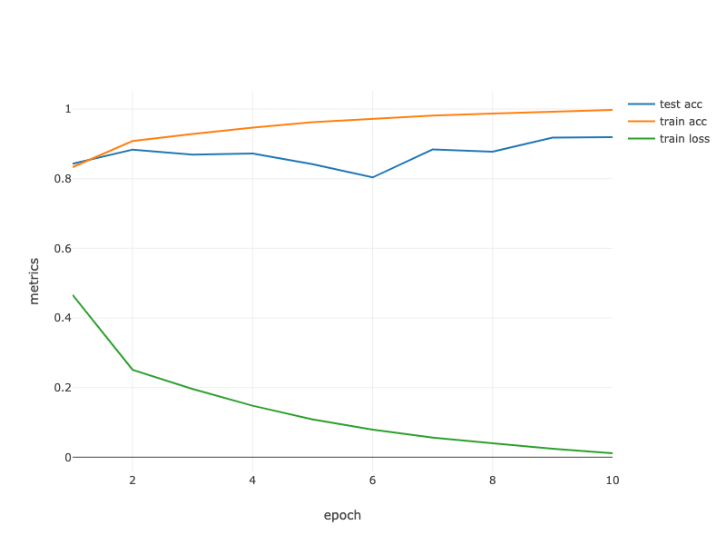
Fig. 7.6.5 Contour Gradient Descent.
String[] lossLabel = new String[trainLoss.length + testAccuracy.length + trainAccuracy.length];

Arrays.fill(lossLabel, 0, trainLoss.length, "train loss");
Arrays.fill(lossLabel, trainAccuracy.length, trainLoss.length + trainAccuracy.length, "train acc");
Arrays.fill(lossLabel, trainLoss.length + trainAccuracy.length,
                trainLoss.length + testAccuracy.length + trainAccuracy.length, "test acc");

Table data = Table.create("Data").addColumns(
            DoubleColumn.create("epoch", ArrayUtils.addAll(epochCount, ArrayUtils.addAll(epochCount, epochCount))),
            DoubleColumn.create("metrics", ArrayUtils.addAll(trainLoss, ArrayUtils.addAll(trainAccuracy, testAccuracy))),
            StringColumn.create("lossLabel", lossLabel)
);

render(LinePlot.create("", data, "epoch", "metrics", "lossLabel"),"text/html");
7.6.5. Summary
Residual blocks allow for a parametrization relative to the identity function \(f(\mathbf{x}) = \mathbf{x}\).
Adding residual blocks increases the function complexity in a well-defined manner.
We can train an effective deep neural network by having residual blocks pass through cross-layer data channels.
ResNet had a major influence on the design of subsequent deep neural networks, both for convolutional and sequential nature.
7.6.6. Exercises
Refer to Table 1 in the [He et al., 2016a] to implement different variants.
For deeper networks, ResNet introduces a “bottleneck” architecture to reduce model complexity. Try to implement it.
In subsequent versions of ResNet, the author changed the “convolution, batch normalization, and activation” architecture to the “batch normalization, activation, and convolution” architecture. Make this improvement yourself. See Figure 1 in [He et al., 2016b] for details.
Prove that if \(\mathbf{x}\) is generated by a ReLU, the ResNet block does indeed include the identity function.
Why cannot we just increase the complexity of functions without bound, even if the function classes are nested?