Run this notebook online:![]() or Colab:
or Colab: ![]()
3.6. Implementation of Softmax Regression from Scratch
Just as we implemented linear regression from scratch, we believe that multiclass logistic (softmax) regression is similarly fundamental and you ought to know the gory details of how to implement it yourself. As with linear regression, after doing things by hand we will breeze through an implementation in DJL for comparison. To begin, let us import the familiar packages.
%load ../utils/djl-imports
%load ../utils/plot-utils.ipynb
%load ../utils/Training.java
%load ../utils/FashionMnistUtils.java
%load ../utils/ImageUtils.java

import ai.djl.basicdataset.cv.classification.FashionMnist;
We will work with the Fashion-MNIST dataset, just introduced in Section 3.5, setting up an iterator with batch size \(256\). We also set it to randomly shuffled elements for each batch for the training set.
int batchSize = 256;
boolean randomShuffle = true;

// get training and validation dataset
FashionMnist trainingSet = FashionMnist.builder()
        .optUsage(Dataset.Usage.TRAIN)
        .setSampling(batchSize, randomShuffle)
        .optLimit(Long.getLong("DATASET_LIMIT", Long.MAX_VALUE))
        .build();

FashionMnist validationSet = FashionMnist.builder()
        .optUsage(Dataset.Usage.TEST)
        .setSampling(batchSize, false)
        .optLimit(Long.getLong("DATASET_LIMIT", Long.MAX_VALUE))
        .build();
3.6.1. Initializing Model Parameters
As in our linear regression example, each example here will be represented by a fixed-length vector. Each example in the raw data is a \(28 \times 28\) image. In this section, we will flatten each image, treating them as \(784\)-long 1D vectors. In the future, we will talk about more sophisticated strategies for exploiting the spatial structure in images, but for now we treat each pixel location as just another feature.
Recall that in softmax regression, we have as many outputs as there are categories. Because our dataset has \(10\) categories, our network will have an output dimension of \(10\). Consequently, our weights will constitute a \(784 \times 10\) matrix and the biases will constitute a \(1 \times 10\) vector. As with linear regression, we will initialize our weights \(W\) with Gaussian noise and our biases to take the initial value \(0\).
int numInputs = 784;
int numOutputs = 10;

NDManager manager = NDManager.newBaseManager();
NDArray W = manager.randomNormal(0, 0.01f, new Shape(numInputs, numOutputs), DataType.FLOAT32);
NDArray b = manager.zeros(new Shape(numOutputs), DataType.FLOAT32);
NDList params = new NDList(W, b);
3.6.2. The Softmax
Before implementing the softmax regression model, let us briefly review
how operators such as sum() work along specific dimensions in an
NDArray. Given a matrix X we can sum over all elements (default)
or only over elements in the same axis, i.e., the column
(new int[]{0}) or the same row (new int[]{1}). We wrap the axis
in an int array since we can specify multiple axes as well. For example
if we call sum() with new int[]{0, 1}, it sums up the elements
over both the rows and columns. In this 2D array, this means the total
sum of the elements within! Note that if X is an array with shape
($2$, $3$) and we sum over the columns (X.sum(new int[]{0})),
the result will be a (1D) vector with shape ($3$,). If we want to
keep the number of axes in the original array (resulting in a 2D array
with shape ($1$, $3$)), rather than collapsing out the dimension
that we summed over we can specify true when invoking sum().
NDArray X = manager.create(new int[][]{{1, 2, 3}, {4, 5, 6}});
System.out.println(X.sum(new int[]{0}, true));
System.out.println(X.sum(new int[]{1}, true));
System.out.println(X.sum(new int[]{0, 1}, true));
ND: (1, 3) gpu(0) int32
[[ 5,  7,  9],
]

ND: (2, 1) gpu(0) int32
[[ 6],
 [15],
]

ND: (1, 1) gpu(0) int32
[[21],
]
We are now ready to implement the softmax function. Recall that softmax
consists of two steps: First, we exponentiate each term (using
exp()). Then, we sum over each row (we have one row per example in
the batch) to get the normalization constants for each example. Finally,
we divide each row by its normalization constant, ensuring that the
result sums to \(1\). Before looking at the code, let us recall how
this looks expressed as an equation:
The denominator, or normalization constant, is also sometimes called the partition function (and its logarithm is called the log-partition function). The origins of that name are in statistical physics where a related equation models the distribution over an ensemble of particles.
public NDArray softmax(NDArray X) {
    NDArray Xexp = X.exp();
    NDArray partition = Xexp.sum(new int[]{1}, true);
    return Xexp.div(partition); // The broadcast mechanism is applied here
}
As you can see, for any random input, we turn each element into a
non-negative number. Moreover, each row sums up to 1, as is required for
a probability. Note that while this looks correct mathematically, we
were a bit sloppy in our implementation because we failed to take
precautions against numerical overflow or underflow due to large (or
very small) elements of the matrix, as we did in
sec_naive_bayes.
NDArray X = manager.randomNormal(new Shape(2, 5));
NDArray Xprob = softmax(X);
System.out.println(Xprob);
System.out.println(Xprob.sum(new int[]{1}));
ND: (2, 5) gpu(0) float32
[[0.1406, 0.117 , 0.5391, 0.0491, 0.1541],
 [0.204 , 0.0605, 0.0759, 0.5691, 0.0905],
]

ND: (2) gpu(0) float32
[1.    , 1.    ]
3.6.3. The Model
Now that we have defined the softmax operation, we can implement the
softmax regression model. The below code defines the forward pass
through the network. Note that we flatten each original image in the
batch into a vector with length numInputs with the reshape()
function before passing the data through our model.
// We need to wrap `net()` in a class so that we can reference the method
// and pass it as a parameter to a function or save it in a variable
public class Net {
    public static NDArray net(NDArray X) {
        NDArray currentW = params.get(0);
        NDArray currentB = params.get(1);
        return softmax(X.reshape(new Shape(-1, numInputs)).dot(currentW).add(currentB));
    }
}
3.6.4. The Loss Function
Next, we need to implement the cross-entropy loss function, introduced in Section 3.4. This may be the most common loss function in all of deep learning because, at the moment, classification problems far outnumber regression problems.
Recall that cross-entropy takes the negative log likelihood of the
predicted probability assigned to the true label
\(-\log P(y \mid x)\). Rather than iterating over the predictions
with a Java for loop (which tends to be inefficient), we can use the
NDArray get() function in conjunction with NDIndex to let us
easily select the appropriate terms from the matrix of softmax entries.
This is typically known as the pick() operator in other frameworks
such as PyTorch. Below, we illustrate the usage on a toy example,
with \(3\) categories and \(2\) examples.
The ":, {}" section of the NDIndex selects all arrays and the
manager.create(new int[]{0, 2}) creates an NDArray with the
values 0 and 2 to pick the 0th and 2nd elements for each respective
NDArray.
Note: when using NDIndex in this way, the passed in NDArray used
for picking indices must be of type int or long. You can use the
toType() function to change the type of the NDArray which will
be shown below.
NDArray yHat = manager.create(new float[][]{{0.1f, 0.3f, 0.6f}, {0.3f, 0.2f, 0.5f}});
yHat.get(new NDIndex(":, {}", manager.create(new int[]{0, 2})));
ND: (2, 2) gpu(0) float32
[[0.1, 0.6],
 [0.3, 0.5],
]
Now we can implement the cross-entropy loss function efficiently with just one line of code.
// Cross Entropy only cares about the target class's probability
// Get the column index for each row
public class LossFunction {
    public static NDArray crossEntropy(NDArray yHat, NDArray y) {
        // Here, y is not guranteed to be of datatype int or long
        // and in our case we know its a float32.
        // We must first convert it to int or long(here we choose int)
        // before we can use it with NDIndex to "pick" indices.
        // It also takes in a boolean for returning a copy of the existing NDArray
        // but we don't want that so we pass in `false`.
        NDIndex pickIndex = new NDIndex()
                 .addAllDim(Math.floorMod(-1, yHat.getShape().dimension()))
                 .addPickDim(y);
        return yHat.get(pickIndex).log().neg();
    }
}
3.6.5. Classification Accuracy
Given the predicted probability distribution yHat, we typically
choose the class with highest predicted probability whenever we must
output a hard prediction. Indeed, many applications require that we
make a choice. Gmail must categorize an email into Primary, Social,
Updates, or Forums. It might estimate probabilities internally, but at
the end of the day it has to choose one among the categories.
When predictions are consistent with the actual category y, they are
correct. The classification accuracy is the fraction of all predictions
that are correct. Although it can be difficult optimize accuracy
directly (it is not differentiable), it is often the performance metric
that we care most about, and we will nearly always report it when
training classifiers.
To compute accuracy we do the following: First, we execute
yHat.argMax(1) where 1 is the axis to gather the predicted classes
(given by the indices for the largest entries in each row). The result
has the same shape as the variable y. Now we just need to check how
frequently the two match. Since the equality function eq() is
datatype-sensitive (e.g., a float32 and a float32 are never
equal), we also need to convert both to the same type (we pick
int32). The result is an NDArray containing entries of 0 (false)
and 1 (true). We then sum the number of true entries and convert the
result to a float. Finally, we get the mean by dividing by the number of
data points.
// Saved in the utils for later use
public float accuracy(NDArray yHat, NDArray y) {
    // Check size of 1st dimension greater than 1
    // to see if we have multiple samples
    if (yHat.getShape().size(1) > 1) {
        // Argmax gets index of maximum args for given axis 1
        // Convert yHat to same dataType as y (int32)
        // Sum up number of true entries
        return yHat.argMax(1).toType(DataType.INT32, false).eq(y.toType(DataType.INT32, false))
            .sum().toType(DataType.FLOAT32, false).getFloat();
    }
    return yHat.toType(DataType.INT32, false).eq(y.toType(DataType.INT32, false))
        .sum().toType(DataType.FLOAT32, false).getFloat();
}
We will continue to use the variables yHat and y defined in the
pick() function, as the predicted probability distribution and
label, respectively. We can see that the first example’s prediction
category is \(2\) (the largest element of the row is \(0.6\)
with an index of \(2\)), which is inconsistent with the actual
label, \(0\). The second example’s prediction category is \(2\)
(the largest element of the row is \(0.5\) with an index of
\(2\)), which is consistent with the actual label, \(2\).
Therefore, the classification accuracy rate for these two examples is
\(0.5\).
NDArray y = manager.create(new int[]{0,2});
accuracy(yHat, y) / y.size();
0.5
Similarly, we can evaluate the accuracy for model net on the dataset
(accessed via dataIterator).
import java.util.function.UnaryOperator;
import java.util.function.BinaryOperator;
// Saved in the utils for future use
public float evaluateAccuracy(UnaryOperator<NDArray> net, Iterable<Batch> dataIterator) {
    Accumulator metric = new Accumulator(2);  // numCorrectedExamples, numExamples
    Batch batch = dataIterator.iterator().next();
    NDArray X = batch.getData().head();
    NDArray y = batch.getLabels().head();
    metric.add(new float[]{accuracy(net.apply(X), y), (float)y.size()});
    batch.close();

    return metric.get(0) / metric.get(1);
}
Here Accumulator is a utility class to accumulate sums over multiple
numbers.
// Saved in utils for future use
/* Sum a list of numbers over time */
public class Accumulator {
    float[] data;

    public Accumulator(int n) {
        data = new float[n];
    }

    /* Adds a set of numbers to the array */
    public void add(float[] args) {
        for (int i = 0; i < args.length; i++) {
            data[i] += args[i];
        }
    }

    /* Resets the array */
    public void reset() {
        Arrays.fill(data, 0f);
    }

    /* Returns the data point at the given index */
    public float get(int index) {
        return data[index];
    }
}
Because we initialized the net model with random weights, the
accuracy of this model should be close to random guessing, i.e.,
\(0.1\) for \(10\) classes.
evaluateAccuracy(Net::net, validationSet.getData(manager));
0.078125
3.6.6. Model Training
The training loop for softmax regression should look strikingly familiar
if you read through our implementation of linear regression in
Section 3.2. Here we refactor the implementation to
make it reusable. First, we define a function to train for one data
epoch. Note that updater() is a general function to update the model
parameters, which accepts the batch size as an argument. Currently, it
is a wrapper of Training.sgd().
@FunctionalInterface
public static interface ParamConsumer {
     void accept(NDList params, float lr, int batchSize);
}

public float[] trainEpochCh3(UnaryOperator<NDArray> net, Iterable<Batch> trainIter, BinaryOperator<NDArray> loss, ParamConsumer updater) {
    Accumulator metric = new Accumulator(3); // trainLossSum, trainAccSum, numExamples

    // Attach Gradients
    for (NDArray param : params) {
        param.setRequiresGradient(true);
    }

    for (Batch batch : trainIter) {
        NDArray X = batch.getData().head();
        NDArray y = batch.getLabels().head();
        X = X.reshape(new Shape(-1, numInputs));

        try (GradientCollector gc = Engine.getInstance().newGradientCollector()) {
            // Minibatch loss in X and y
            NDArray yHat = net.apply(X);
            NDArray l = loss.apply(yHat, y);
            gc.backward(l);  // Compute gradient on l with respect to w and b
            metric.add(new float[]{l.sum().toType(DataType.FLOAT32, false).getFloat(),
                                   accuracy(yHat, y),
                                   (float)y.size()});
            gc.close();
        }
        updater.accept(params, lr, batch.getSize());  // Update parameters using their gradient

        batch.close();
    }
    // Return trainLoss, trainAccuracy
    return new float[]{metric.get(0) / metric.get(2), metric.get(1) / metric.get(2)};
}
Before showing the implementation of the training function, we define a utility class that draws data in animation. Again, it aims to simplify the code in later chapters.
import tech.tablesaw.api.Row;
import tech.tablesaw.columns.Column;

// Saved in utils
/* Animates a graph with real-time data. */
class Animator {
    private String id; // Id reference of graph(for updating graph)
    private Table data; // Data Points

    public Animator() {
        id = "";

        // Incrementally plot data
        data = Table.create("Data")
        .addColumns(
            FloatColumn.create("epoch", new float[]{}),
            FloatColumn.create("value", new float[]{}),
            StringColumn.create("metric", new String[]{})
        );
    }

    // Add a single metric to the table
    public void add(float epoch, float value, String metric) {
        Row newRow = data.appendRow();
        newRow.setFloat("epoch", epoch);
        newRow.setFloat("value", value);
        newRow.setString("metric", metric);
    }

    // Add accuracy, train accuracy, and train loss metrics for a given epoch
    // Then plot it on the graph
    public void add(float epoch, float accuracy, float trainAcc, float trainLoss) {
        add(epoch, trainLoss, "train loss");
        add(epoch, trainAcc, "train accuracy");
        add(epoch, accuracy, "test accuracy");
        show();
    }

    // Display the graph
    public void show() {
        if (id.equals("")) {
            id = display(LinePlot.create("", data, "epoch", "value", "metric"));
            return;
        }
        update();
    }

    // Update the graph
    public void update() {
        updateDisplay(id, LinePlot.create("", data, "epoch", "value", "metric"));
    }

    // Returns the column at the given index
    // if it is a float column
    // Otherwise returns null
    public float[] getY(Table t, int index) {
        Column c = t.column(index);
        if (c.type() == ColumnType.FLOAT) {
            float[] newArray = new float[c.size()];
            System.arraycopy(c.asList().toArray(), 0, newArray, 0, c.size());
            return newArray;
        }
        return null;
    }
}
The training function then runs multiple epochs and visualize the training progress.
public void trainCh3(UnaryOperator<NDArray> net, Dataset trainDataset, Dataset testDataset,
                     BinaryOperator<NDArray> loss, int numEpochs, ParamConsumer updater)
                                                            throws IOException, TranslateException {
    Animator animator = new Animator();
    for (int i = 1; i <= numEpochs; i++) {
        float[] trainMetrics = trainEpochCh3(net, trainDataset.getData(manager), loss, updater);
        float accuracy = evaluateAccuracy(net, testDataset.getData(manager));
        float trainAccuracy = trainMetrics[1];
        float trainLoss = trainMetrics[0];

        animator.add(i, accuracy, trainAccuracy, trainLoss);
        System.out.printf("Epoch %d: Test Accuracy: %f\n", i, accuracy);
        System.out.printf("Train Accuracy: %f\n", trainAccuracy);
        System.out.printf("Train Loss: %f\n", trainLoss);
    }
}
Again, we use the minibatch stochastic gradient descent to optimize the
loss function of the model. Note that the number of epochs
(numEpochs), and learning rate (lr) are both adjustable
hyper-parameters. By changing their values, we may be able to increase
the classification accuracy of the model. In practice we will want to
split our data three ways into training, validation, and test data,
using the validation data to choose the best values of our
hyper-parameters.
int numEpochs = 5;
float lr = 0.1f;

public class Updater {
    public static void updater(NDList params, float lr, int batchSize) {
        Training.sgd(params, lr, batchSize);
    }
}

trainCh3(Net::net, trainingSet, validationSet, LossFunction::crossEntropy, numEpochs, Updater::updater);
Epoch 1: Test Accuracy: 0.820313
Train Accuracy: 0.750000
Train Loss: 0.783057
Epoch 2: Test Accuracy: 0.816406
Train Accuracy: 0.814083
Train Loss: 0.570253
Epoch 3: Test Accuracy: 0.828125
Train Accuracy: 0.825600
Train Loss: 0.525173
Epoch 4: Test Accuracy: 0.839844
Train Accuracy: 0.831117
Train Loss: 0.501283
Epoch 5: Test Accuracy: 0.859375
Train Accuracy: 0.836683
Train Loss: 0.485033
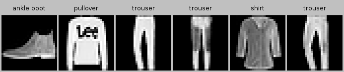
3.6.7. Prediction
Now that training is complete, our model is ready to classify some images. Given a series of images, we will compare their actual labels (first line of text output) and the model predictions (second line of text output).
// Saved in the FashionMnistUtils class for later use
// Number should be < batchSize for this function to work properly
public BufferedImage predictCh3(UnaryOperator<NDArray> net, ArrayDataset dataset, int number, NDManager manager)
    throws IOException, TranslateException {
    int[] predLabels = new int[number];

    Batch batch = dataset.getData(manager).iterator().next();
    NDArray X = batch.getData().head();
    int[] yHat = net.apply(X).argMax(1).toType(DataType.INT32, false).toIntArray();
    for (int i = 0; i < number; i++) {
        predLabels[i] = yHat[i];
    }

    return FashionMnistUtils.showImages(dataset, predLabels, 28, 28, 4, manager);
}

predictCh3(Net::net, validationSet, 6, manager)
3.6.8. Summary
With softmax regression, we can train models for multi-category classification. The training loop is very similar to that in linear regression: retrieve and read data, define models and loss functions, then train models using optimization algorithms. As you will soon find out, most common deep learning models have similar training procedures.
3.6.9. Exercises
In this section, we directly implemented the softmax function based on the mathematical definition of the softmax operation. What problems might this cause (hint: try to calculate the size of \(\exp(50)\))?
The function
crossEntropy()in this section is implemented according to the definition of the cross-entropy loss function. What could be the problem with this implementation (hint: consider the domain of the logarithm)?What solutions you can think of to fix the two problems above?
Is it always a good idea to return the most likely label. E.g., would you do this for medical diagnosis?
Assume that we want to use softmax regression to predict the next word based on some features. What are some problems that might arise from a large vocabulary?